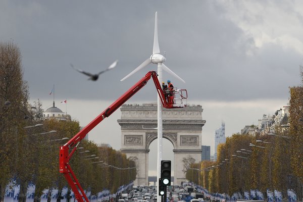
 Figure 1 – New windmill being installed on the Champs-Élysées in Paris
(Photo by Patrick Kovarik/Agence France-Presse — Getty Images)
This blog will be posted one day after the scheduled opening of the COP21 meeting in Paris. The last two blogs, which I dedicated to this conference, also addressed the ramifications of the terrorist attack that happened on Friday, November 13.
This blog is going to be a bit longer than usual because in addition to further discussing the consequences of the attack, I need to conclude my description of the methods being used to measure and report greenhouse gas levels, since that will be a central topic of discussions during the conference.
Following the attack, the French government declared that the meeting would take place as planned but with a considerable tightening of security. As a result, all of the major demonstrations that environmental groups had scheduled for Sunday were cancelled, upsetting a large number of people worldwide. One response to this ban included setting up over 22,000 pairs of donated shoes in the Place de la Republique to “stand in” for a fraction the masses that would have otherwise attended (estimated 200,000-500,000). UN Secretary-General Ban Ki-moon and Pope Francis even sent a pair each!
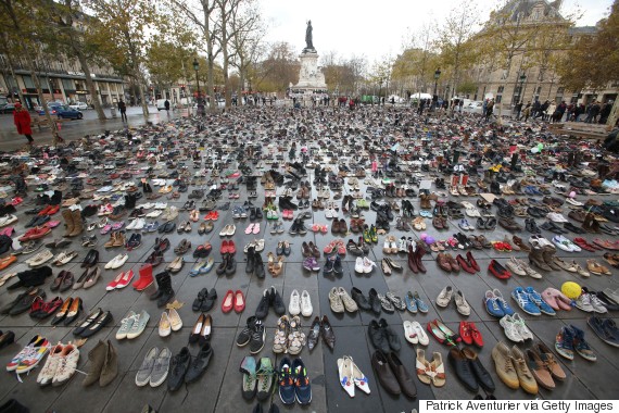 Figure 2 – Shoes placed in Place de la Republique in Paris. (Photo by Patrick Aventurier/Getty Images)
The success of the conference has gathered new urgency as many have reemphasized the connections between warming temperatures and the Syrian civil war. That war has not only resulted in millions of refugees but has also been the cause (according to many) of an increase in the global spread of terrorism. In light of the recent Paris attacks, this problem is at the forefront of the public consciousness. This also means that an objective that many (but not all) at the conference share is to produce an effective agreement to limit anthropogenic contributions to the warming.
Negotiations during the conference are expected to focus on the two main aspects of dealing with anthropogenic global climate change: mitigation of human impact on the climate through changes in the chemistry of the atmosphere and adaptation to those changes that are already taking place (e.g. severe droughts, rising ocean levels, etc.) and will be amplified in the coming years.
Background – The Keeling and Whorf Curve:
Focus on the human impact on climate change started with measurements of the Keeling Whorf curve, a modern version of which is shown in Figure 3.
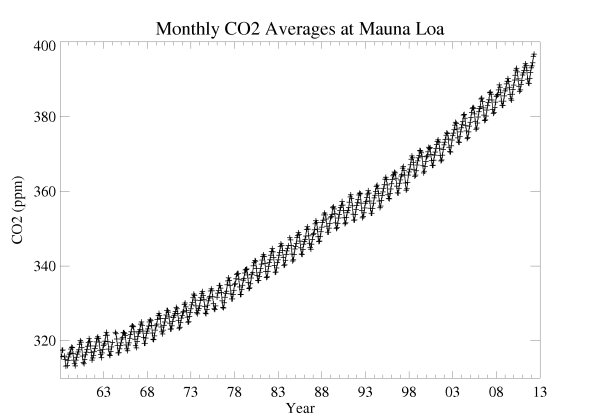 Figure 3 – A recent version of the Keeling and Whorf curve that measures the carbon dioxide concentrations as observed at Mauna Loa, Hawaii.
The original Keeling and Whorf measurements were collected continuously from the same location in Hawaii, starting in 1958. Samples of air were collected four times a day, and the concentration of carbon dioxide was measured by infrared absorption spectroscopy. The measurements showed a steady increase in the concentration of carbon dioxide at the site. Since the original measurements, the monitoring has expanded to other sites at different latitudes. The pattern of a monotonic increase in the carbon concentration is found at every site. You can, for instance, compare the pattern above with the data obtained by NASA through the OCO-2 satellite measurements, as shown in last week’s blog. However, Figure 3 also shows something else: superimposed on the steady CO2 concentrations in Mauna Loa are very regular oscillations. Such oscillations are absent from similar measurements taken in Antarctica and they vary with the latitude of the site. These oscillations directly exemplify the yearly cycle and the difference between each site’s carbon dioxide source and its sink. The fluctuations represent the full complexities of the carbon cycle as it equilibrates between the land, the air, and the ocean. The yearly cycles shown in Figure 3 were attributed to the large percentage of trees in the northern hemisphere that shed their leaves in the fall and regrow them in the spring. The corresponding result is that less carbon dioxide is captured during the winter than in the summer.
Present Practices:
Unlike the satellite measurements that were described in last week’s blog and the Keeling and Whorf measurements, the IPCC guidelines are not based on direct measurements of carbon dioxide or other greenhouse gases. Instead, they focus on the sources (primarily but not exclusively energy sources) of the greenhouse gases. This completely eliminates the issue of attempting to distinguish between anthropogenic sources and natural sources but they rely fully on our full understanding of the science of these sources and full reliance on the performance of governments.
The current measurement and reporting practices are anchored on guidelines that were issued by the IPCC (International Panel on Climate Change) in 2006, and the periodic (almost annual) updates that the same institution issues.
 Figure 3 – Coverpages of the IPCC 2006 guidelines for measurements and reporting of greenhouse gases.
These guidelines came in the form of 5 volumes:
Volume 1 (red) – General Guidelines and Reporting (GGR).
Volume 2 (yellow) – Energy
Volume 3 (green) – Industrial Processing and Product Use (IPPU).
Volume 4 (blue) – Agriculture, Forestry and Other Land Use (AFOLU).
Volume 5 (violet) – Waste
Volume 1 includes a short description about the concepts involved in these guidelines:
1 INTRODUCTION TO THE 2006 GUIDELINES
The 2006 IPCC Guidelines for National Greenhouse Gas Inventories (2006 Guidelines) were produced at the invitation of the United Nations Framework Convention on Climate Change (UNFCCC) to update the Revised 1996 Guidelines and associated good practice guidance1 which provide internationally agreed2 methodologies intended for use by countries to estimate greenhouse gas inventories to report to the UNFCCC. This chapter provides an introduction to the 2006 Guidelines for a broad range of users, including countries and inventory compilers setting out to prepare inventory estimates for the first time. Sections 1.1 to 1.3 describe the overarching framework of these Guidelines, focusing on scope, approach, and structure. Sections 1.4 through 1.5 present step-by-step guidance on how to use the 2006 Guidelines for compiling a greenhouse gas inventory.
1.1 CONCEPTS
Inventories rely on a few key concepts for which there is a common understanding. This helps ensure that inventories are comparable between countries, do not contain double counting or omissions, and that the time series reflect actual changes in emissions.
Anthropogenic emissions and removals
Anthropogenic emissions and removals means that greenhouse gas emissions and removals included in national inventories are a result of human activities. The distinction between natural and anthropogenic emissions and removals follows straightforwardly from the data used to quantify human activity. In the Agriculture, Forestry and Other Land Use (AFOLU) Sector, emissions and removals on managed land are taken as a proxy for anthropogenic emissions and removals, and inter annual variations in natural background emissions and removals, though these can be significant, are assumed to average out over time.
National territory
National inventories include greenhouse gas emissions and removals taking place within national territory and offshore areas over which the country has jurisdiction. There are some special issues that are described in Section 8.2.1 of Volume 1. For example, emissions from fuel use in road transport is included in the emissions of the country where the fuel is sold and not where the vehicle is driven, as fuel sale statistics are widely available and usually much more accurate.
Inventory year and time series
National inventories contain estimates for the calendar year during which the emissions to (or removals from) the atmosphere occur. Where suitable data to follow this principle are missing, emissions/removals may be estimated using data from other years applying appropriate methods such as averaging, interpolation and extrapolation. A sequence of annual greenhouse gas inventory estimates (e.g., each year from 1990 to 2000) is called a time series. Because of the importance of tracking emissions trends over time, countries should ensure that a time series of estimates is as consistent as possible.
Inventory reporting
A greenhouse gas inventory report includes a set of standard reporting tables covering all relevant gases, categories and years, and a written report that documents the methodologies and data used to prepare the estimates. The 2006 Guidelines provide standardized reporting tables, but the actual nature and content of the tables and written report may vary according to, for example, a country’s obligations as a Party to the UNFCCC. The 2006 Guidelines provide worksheets to assist with the transparent application of the most basic (or Tier 1)
1.2 ESTIMATION METHODS
As with the 1996 Guidelines and IPCC Good Practice Guidance the most common simple methodological approach is to combine information on the extent to which a human activity takes place (called activity data or AD) with coefficients which quantify the emissions or removals per unit activity. These are called emission factors (EF). The basic equation is therefore:
Emissions = AD • EF
For example, in the energy sector fuel consumption would constitute activity data, and mass of carbon dioxide emitted per unit of fuel consumed would be an emission factor. The basic equation can in some circumstances be modified to include other estimation parameters than emission factors. Where time lags are involved, due for example to the time it takes for material to decompose in a landfill or leakage of refrigerants from cooling devices, other methods are provided, for example first order decay methods. The 2006 Guidelines also allow for more complex modelling approaches, particularly at higher tiers. Though this simple equation is widely used, the 2006 Guidelines also contain mass balance methods, for example the stock change methods used in the AFOLU sector which estimates CO2 emissions from changes over time in carbon content of living biomass and dead organic matter pools. Carbon dioxide from the combustion or decay of short-lived biogenic material removed from where it was grown is reported as zero in the Energy, IPPU and Waste Sectors (for example CO2 emissions from iofuels6,7, and CO2 emissions from biogenic material in Solid Waste Disposal Sites (SWDS)). In the AFOLU Sector, when using Tier 1 methods for short lived products, it is assumed that the emission is balanced by carbon uptake prior to harvest, within the uncertainties of the estimates, so the net emission is zero. Where higher Tier estimation shows that this emission is not balanced by a carbon removal from the atmosphere, this net emission or removal should be included in the emission and removal estimates for AFOLU Sector through carbon stock change estimates. Material with long lifetime is dealt with in the HWP section.
IPCC methods use the following concepts:
Good Practice: In order to promote the development of high quality national greenhouse gas inventories a collection of methodological principals, actions and procedures were defined in the previous guidelines and collectively referred to as good practice. The 2006 Guidelines retain the concept of good practice including the definition introduced with GPG2000. This has achieved general acceptance amongst countries as the basis for inventory development and says that inventories consistent with good practice are those which contain neither over- nor under-estimates so far as can be judged, and in which uncertainties are reduced as far as practicable.
Tiers: A tier represents a level of methodological complexity. Usually three tiers are provided. Tier 1 is the basic method, Tier 2 intermediate and Tier 3 most demanding in terms of complexity and data requirements. Tiers 2 and 3 are sometimes referred to as higher tier methods and are generally considered to be more accurate.
Default data: Tier 1 methods for all categories are designed to use readily available national or international statistics in combination with the provided default emission factors and additional parameters that are provided, and therefore should be feasible for all countries.
Key Categories: The concept of key category8 is used to identify the categories that have a significant influence on a country’s total inventory of greenhouse gases in terms of the absolute level of emissions and removals, the trend in emissions and removals, or uncertainty in emissions and removals. Key Categories should be the priority for countries during inventory resource allocation for data collection, compilation, quality assurance/quality control and reporting.
In future blogs, I will be able to shift from speculations to assessments, as we try to understand and explain the various prevailing currents at the conference.