My previous blog cited a long 2016 report by the National Academy that outlines two classes of mechanisms used for climate events to assess the likelihood of attributions to climate change:
Event attribution approaches can be generally divided into two classes: (1) those that rely on the observational record to determine the change in probability or magnitude of events, and (2) those that use model simulations to compare the manifestation of an event in a world with human-caused climate change to that in a world without. Most studies use both observations and models to some extent—for example, modeling studies will use observations to evaluate whether models reproduce the event of interest and whether the mechanisms involved correspond to observed mechanisms, and observational studies may rely on models for attribution of the observed changes.
Below that paragraph, I showed a table from the same report that illustrated the state of understanding of various extreme consequences of climate change. These were grouped into three relevant categories:
- Ability to model the climate event.
- Quality and length of observational record of the event
- Understanding the mechanisms that lead to the event.
In all three categories, the only events for which the paper claimed to have a high degree of understanding were extremely high and low temperatures. Amid the fires, droughts, extreme storms, etc., the report’s table doesn’t even mention floods as a distinctive category.
Plenty of work remains for us to quantify the understanding of climate change’s impact on these extreme weather phenomena. In future blogs, I will try to describe in more detail some of the difficulties involved in quantifying such attribution.
This blog is focused on two relevant aspects: Attribution to anthropogenic (human-caused) to global extreme climate events and a distinction between chaotic systems, on which physics teaches us that initial conditions for such events cannot be determined, and anthropogenic attributions to such events.
I have repeatedly discussed anthropogenic attributions to global extreme climate events in previous blogs. The two that are most relevant are the following:
“Doomsday: Attributions,” from October 3, 2017, deals with the modeling of human influence on the global temperature from the beginning of the 20th century and the decline of the radioactive isotope carbon-14 in the atmosphere over that time—an indicator that burning fossil fuels is culpable of that change.
“The Little Ice Age,” from April 16, 2019, shows the reconstructed global temperature change from the beginning of the common era to the present day. This reconstruction shows a “hockey stick” shape: behavior with sharp temperature rises from the mid-20th century.
These data are such important evidence that they have convinced more than 90% of the world’s scientists about the post-Industrial Revolution climate change’s major human attribution. They also satisfy the two classes of observation outlined by the National Academy in last week’s blog. Figure 1 is repeated from the October 3, 2017, blog, showing the NASA simulation of the global temperature from the beginning of the 20th century.
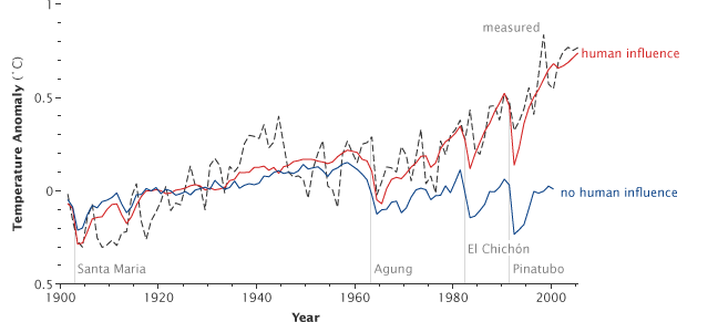
Figure 1 – Attribution of global warming – simulation of 20th century global mean temperatures (with and without human influences) compared to observations
(Source: NASA via Wikipedia)
Chaos
The Oxford Language Dictionary defines chaos in the following way:
PHYSICS
- behavior so unpredictable as to appear random, owing to great sensitivity to small changes in conditions.
- the formless matter supposed to have existed before the creation of the universe.
I will focus here on the first definition (I covered the second definition in my July 26, 2022 blog, “Creation”).
When you Google climate change attributions and chaos, you will get many links to climate change deniers who claim that since—per definition—chaotic systems are very sensitive to initial conditions, we cannot attribute the majority of climate change to humans and that climate change cannot be predicted and thus cannot be attributed. Skeptical Science is a famous blog that addresses and rebuts such issues; I have mentioned it several times, including in one of my earliest blogs (July 13, 2013). I am quoting the relevant Skeptical Science post on this issue below.
The argument: Climate is chaotic and cannot be predicted
‘Lorenz (1963), in the landmark paper that founded chaos theory, said that because the climate is a mathematically-chaotic object (a point which the UN’s climate panel admits), accurate long-term prediction of the future evolution of the climate is not possible “by any method”. At present, climate forecasts even as little as six weeks ahead can be diametrically the opposite of what actually occurs, even if the forecasts are limited to a small region of the planet.’ (Christopher Monckton)
Response (with repeating Monckton’s argument): “One of the defining traits of a chaotic system is ‘sensitive dependence to initial conditions’. This means that even very small changes in the state of the system can quickly and radically change the way that the system develops over time. Edward Lorenz’s landmark 1963 paper demonstrated this behavior in a simulation of fluid turbulence, and ended hopes for long-term weather forecasting.”
However, climate is not weather, and modeling is not forecasting.
Although it is generally not possible to predict a specific future state of a chaotic system (there is no telling what temperature it will be in Oregon on December 21 2012), it is still possible to make statistical claims about the behavior of the system as a whole (it is very likely that Oregon’s December 2012 temperatures will be colder than its July 2012 temperatures). There are chaotic components to the climate system, such as El Nino and fluid turbulence, but they all have much less long-term influence than the greenhouse effect. It’s a little like an airplane flying through stormy weather: It may be buffeted around from moment to moment, but it can still move from one airport to another.
Nor do climate models generally produce weather forecasts. Models often run a simulation multiple times with different starting conditions, and the ensemble of results are examined for common properties (one example: Easterling & Wehner 2009). This is, incidentally, a technique used by mathematicians to study the Lorenz functions.
The chaotic nature of turbulence is no real obstacle to climate modeling, and it does not negate the existence or attribution of climate change.
Wikipedia’s entry summarizes the essentials of chaos theory:
Chaos theory is an interdisciplinary scientific theory and branch of mathematics focused on underlying patterns and deterministic laws, of dynamical systems, that are highly sensitive to initial conditions, that were once thought to have completely random states of disorder and irregularities.[1] Chaos theory states that within the apparent randomness of chaotic complex systems, there are underlying patterns, interconnection, constant feedback loops, repetition, self-similarity, fractals, and self-organization.[2] The butterfly effect, an underlying principle of chaos, describes how a small change in one state of a deterministic nonlinear system can result in large differences in a later state (meaning that there is sensitive dependence on initial conditions).[3] A metaphor for this behavior is that a butterfly flapping its wings in Brazil can cause a tornado in Texas.
The simplest way to get a feeling for or understanding of chaos theory is to play with the logistic map:
The logistic map is a polynomial mapping (equivalently, recurrence relation) of degree 2, often cited as an archetypal example of how complex, chaotic behavior can arise from very simple non-linear dynamical equations. The map was popularized in a 1976 paper by the biologist Robert May,[1] in part as a discrete-time demographic model analogous to the logistic equation written down by Pierre François Verhulst.[2] Mathematically, the logistic map is written
where xn is a number between zero and one, that represents the ratio of existing population to the maximum possible population. This nonlinear difference equation is intended to capture two effects:
- reproduction where the population will increase at a rate proportional to the current population when the population size is small.
- starvation (density-dependent mortality) where the growth rate will decrease at a rate proportional to the value obtained by taking the theoretical “carrying capacity” of the environment less the current population.
The usual values of interest for the parameter are those in the interval [0, 4], so that xn remains bounded on [0, 1]. The r = 4 case of the logistic map is a nonlinear transformation of both the bit-shift map and the μ = 2 case of the tent map. If r > 4 this leads to negative population sizes. (This problem does not appear in the older Ricker model, which also exhibits chaotic dynamics.) One can also consider values of r in the interval [−2, 0], so that xn remains bounded on [−0.5, 1.5].[3]
By varying the parameter r, the following behavior is observed:
Evolution of different initial conditions as a function of r
-
With r between 0 and 1, the population will eventually die, independent of the initial population.
-
With r between 1 and 2, the population will quickly approach the value r − 1/r, independent of the initial population.
-
With r between 2 and 3, the population will also eventually approach the same value r − 1/r, but first will fluctuate around that value for some time. The rate of convergence is linear, except for r = 3, when it is dramatically slow, less than linear (see Bifurcation memory).
-
With r between 3 and 1 + √6≈ 3.44949 the population will approach permanent oscillations between two values. These two values are dependent on r and given by[3]
-
With r between 3.44949 and 3.54409 (approximately), from almost all initial conditions the population will approach permanent oscillations among four values. The latter number is a root of a 12th degree polynomial (sequence A086181 in the OEIS).
-
With r increasing beyond 3.54409, from almost all initial conditions the population will approach oscillations among 8 values, then 16, 32, etc. The lengths of the parameter intervals that yield oscillations of a given length decrease rapidly; the ratio between the lengths of two successive bifurcation intervals approaches the Feigenbaum constant δ ≈ 4.66920. This behavior is an example of a period-doubling cascade.
-
At r ≈ 3.56995 (sequence A098587 in the OEIS) is the onset of chaos, at the end of the period-doubling cascade. From almost all initial conditions, we no longer see oscillations of finite period. Slight variations in the initial population yield dramatically different results over time, a prime characteristic of chaos.
The result of all of this is shown in Figure 2:
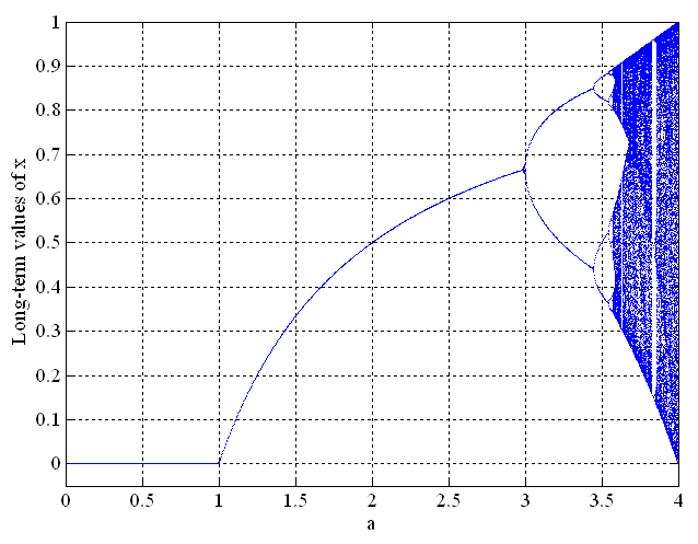
Figure 2 – Logistic map of Equation 1, regarding global population (Source: Hyperchaos)
The easiest way to construct Figure 2 from Equation 1 is to put the values of the three parameters of Equation 1 into Excel and to take about 30 recurring values of x.
Figure 2 starts with a deterministic pattern and continues, independent of the initial conditions until the rate (r in Equation 1 or a in Figure 2) reaches the value of 3. As the value of the rate surpasses 3, it starts to bifurcate—first between two very different values, then between other values—into patterns that look completely random. In practice, this means that major population changes can follow the smallest changes in the initial conditions. If we are in that chaotic regime, we cannot trace our way back to where we started the process.
The organization Project Nile published a great piece about chaos theory.
When we have an extreme weather event such as a fire or flood, we often look for a source that we can blame. This might satisfy our instincts but it will not be useful. On the other hand, if we can compare the statistics in terms of frequency and intensity to a missing driving force (like human action), as we are trying to do with attribution research, we can begin mitigation efforts and work to lessen the rate of such events.
This conclusion agrees with the Skeptical Science conclusion: “attribution is not a determination of initial conditions.”
Personally, I think the chaos theory itself is relatively flawed, as for something to be truly chaotic, it would mean it has no way to actually be predicted. I think the proper term would be “inconsistent” which is a term that could be applied to various parts of climate.
Climate change makes a huge impact on our world. Things such as weather is constantly changing, same way that things are happening every minute which makes it constant. How can we predict what will happen next? The answer to that is we can’t. It’s just unpredictable.
As stated in the blog, “ Plenty of work remains for us to quantify the understanding of climate change’s impact on these extreme weather phenomena.” This is because it might have a huge impact on our world. For example, the superior weather changes every day. On one day it can be hot and on another day it could be cold. It’s just that we can’t predict what will happen.
The blog has mentioned that “ Plenty of work remains for us to quantify the understanding of climate change’s impact on these extreme weather phenomena” because all we can still make are guesses, predictions and assumptions about what probably can happen to our planet and all its life forms due to climate change, so there’s no absolute true prediction but there’s still a certainty that things will only continue to get worse and who knows it might just be even more catastrophic than what is being predicted at the moment. In my opinion the predictions that we were able to conclude are scary but the fact that they aren’t 100% true because the consequences could be far greater than anticipated is even more terrifying.
According to Climate.NASA.gov, it states: “Scientific information taken from natural sources (such as ice cores, rocks, and tree rings) and from modern equipment (like satellites and instruments) all show the signs of a changing climate. From global temperature rise to melting ice sheets, the evidence of a warming planet abounds.” This essentially captures the unheard-of transformation of events taking place in the 20th century. The rate and extent of the ozone layer’s decline have also been determined by scientists.